theta_params <- thetas
omega_sigma_params <- rest[str_detect(rest, "omega|sigma")]
other_params <- rest[str_detect(rest, "nu")]
sigma_params <- c("sigma[1]", "sigma[2]")
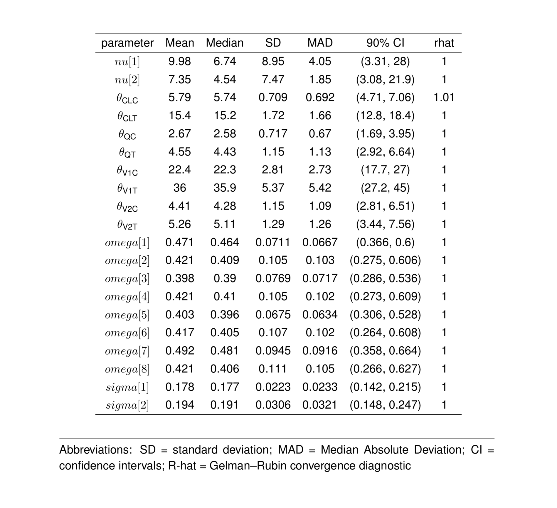
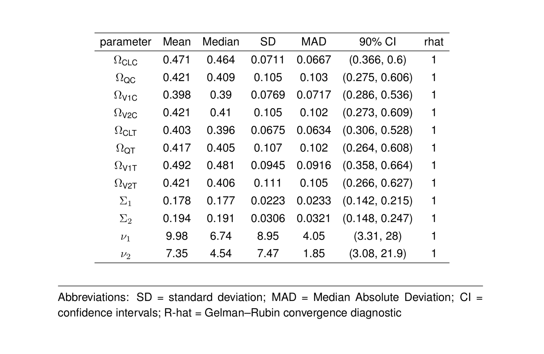
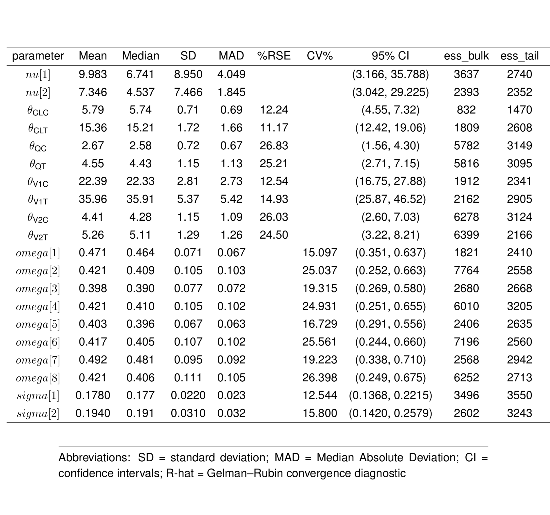
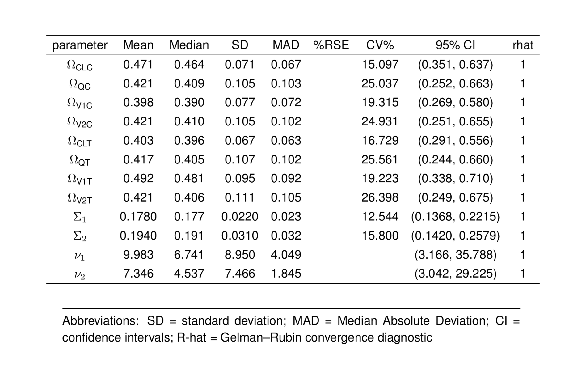
footAbbrev <- "Abbreviations: SD = standard deviation; MAD = Median Absolute Deviation; CI = confidence intervals; R-hat = Gelman–Rubin convergence diagnostic"
pars <- c("lp__", pars1)
draws <- mod5_res$draws(pars)
sig <- function(x, digits=2) round(x, digits)
ptable_all <- summarise_draws(
draws,
mean,
median,
sd,
mad,
q2.5 = ~quantile(.x, 0.025),
q5 = ~quantile(.x, 0.05),
q95 = ~quantile(.x, 0.95),
q97.5 = ~quantile(.x, 0.975),
ess_bulk,
ess_tail,
rhat) %>%
rename(parameter = variable) %>%
mutate(
`%RSE` = if_else(mean != 0, (sd / mean) * 100, NA_real_),
`CV%` = if_else(parameter %in% omega_sigma_params & mean != 0, (sd / mean) * 100, NA_real_)) %>%
mutate(
`%RSE` = if_else(parameter %in% theta_params, formatC(`%RSE`, format = "f", digits = 2), NA_character_),
`CV%` = if_else(parameter %in% omega_sigma_params, formatC(`CV%`, format = "f", digits = 3), NA_character_)) %>%
mutate(
mean = if_else(parameter %in% theta_params, formatC(mean, format = "f", digits = 2),
formatC(mean, format = "f", digits = 3)),
median= if_else(parameter %in% theta_params, formatC(median, format = "f", digits = 2),
formatC(median, format = "f", digits = 3)),
sd = if_else(parameter %in% theta_params, formatC(sd, format = "f", digits = 2),
formatC(sd, format = "f", digits = 3)),
mad = if_else(parameter %in% theta_params, formatC(mad, format = "f", digits = 2),
formatC(mad, format = "f", digits = 3)),
`%RSE`= if_else(parameter %in% theta_params, formatC(`%RSE`, format = "f", digits = 2), `%RSE`),
`CV%` = if_else(parameter %in% omega_sigma_params, formatC(`CV%`, format = "f", digits = 2), `CV%`),
`2.5%` = if_else(parameter %in% theta_params,
formatC(as.numeric(`2.5%`), format = "f", digits = 2),
if_else(parameter %in% sigma_params,
formatC(as.numeric(`2.5%`), format = "f", digits = 4),
formatC(as.numeric(`2.5%`), format = "f", digits = 3))),
`5%` = if_else(parameter %in% theta_params,
formatC(as.numeric(`5%`), format = "f", digits = 2),
if_else(parameter %in% sigma_params,
formatC(as.numeric(`5%`), format = "f", digits = 4),
formatC(as.numeric(`5%`), format = "f", digits = 3))),
`95%` = if_else(parameter %in% theta_params,
formatC(as.numeric(`95%`), format = "f", digits = 2),
if_else(parameter %in% sigma_params,
formatC(as.numeric(`95%`), format = "f", digits = 4),
formatC(as.numeric(`95%`), format = "f", digits = 3))),
`97.5%` = if_else(parameter %in% theta_params,
formatC(as.numeric(`97.5%`), format = "f", digits = 2),
if_else(parameter %in% sigma_params,
formatC(as.numeric(`97.5%`), format = "f", digits = 4),
formatC(as.numeric(`97.5%`), format = "f", digits = 3)))) %>%
mutate(across(c("mean", "sd", "2.5%", "97.5%"),
~if_else(parameter %in% c("sigma[1]", "sigma[2]"),
formatC(as.numeric(.), format = "f", digits = 4), .))) %>%
mutate(`90% CI` = paste0("(", `5%`, ", ", `95%`, ")"),
`95% CI` = paste0("(", `2.5%`, ", ", `97.5%`, ")")) %>%
mutate(ess_bulk = round(ess_bulk, 0), ess_tail = round(ess_tail,0), rhat = round(rhat, 2)) %>%
select(parameter, mean, median, sd, mad, `%RSE`, `CV%`, `95% CI`, ess_bulk, ess_tail, rhat) #`90% CI`,
gtGreek <- function(text) {
case_when(
text %in% c("CLC", "QC", "V1C", "V2C", "CLT", "QT", "V1T", "V2T") ~
paste0("\\theta_{\\text{", text, "}}"),
text == "omega" ~ "\\Omega",
text == "sigma" ~ "\\Sigma",
text == "nu" ~ "\\nu",
TRUE ~ text
)
}
mathMode <- function(x) paste0("$", x, "$")
formatGreekNames <- function(df) {
df %>%
mutate(is_theta = str_ends(parameter, "Hat$"),
base = if_else(is_theta, str_remove(parameter, "Hat$"), parameter)) %>%
mutate(greek = mathMode(gtGreek(base))) %>%
select(parameter = greek,
mean, median, sd, mad, `%RSE`, `CV%`, `95% CI`, ess_bulk, ess_tail, rhat) #`90% CI`,
}
ptable1_greek <- ptable_all %>%
filter(parameter %in% thetas) %>%
formatGreekNames()
ptable2_greek <- ptable_all %>%
filter(parameter %in% rest) %>%
formatGreekNames()
param_df <- bind_rows(ptable1_greek, ptable2_greek) %>%
arrange(!str_detect(parameter, "Omega|Sigma|nu"), parameter)
fixed <- param_df %>%
st_new() %>%
st_center(desc = col_ragged(6.5), abb = "l") %>%
st_rename("Mean" = "mean", "Median" = "median", "SD" = "sd", "MAD" = "mad") %>%
st_blank("abb", "greek", "desc") %>%
st_files(r = NULL) %>%
st_notes(footAbbrev) %>%
st_noteconf(type = "minipage") %>%
stable()