Code
knitr::opts_chunk$set(message = FALSE, warning = FALSE)
#renv::snapshot()
renv::status()
This project does not appear to be using renv.
Use `renv::init()` to initialize the project.Antimicrobial therapy requires a precise dosage of antibiotics to achieve the therapeutic goal with a minimum level of toxic effects and low risk of developing microbial resistance. Due to the altered pharmacokinetics of drugs in critically ill patients, the dosing regimen in this group of patients may differ from the dosing regimen established in clinical trials on healthy volunteers. Ceftolozane with tazobactam is administered during therapy in patients with particularly resistant strains, especially Pseudomonas aeruginosa. Administration of antibiotics requires precise dosing. Reaching concentrations too low than needed to inhibit growth or kill the bacteria can lead to the development of antibiotic resistance. Reaching too high doses is also dangerous because it can lead to severe side effects and organ damage.
knitr::opts_chunk$set(message = FALSE, warning = FALSE)
#renv::snapshot()
renv::status()This project does not appear to be using renv.
Use `renv::init()` to initialize the project.#load library
# repos <- c("https://metrumresearchgroup.github.io/r_validated", options()$repos)
# install.packages("mrggsave", repos = unique(repos), type = "source", destdir = NULL)
library(pracma)
library(dplyr)
library(ggplot2)
library(patchwork)
library(mrgsolve)
library(naniar)
library(knitr)
library(data.table)
library(tidyverse)
library(glue)
library(whisker)
library(here)
library(scales)
library(pmplots)
library(pmtables)
library(nmrec)
library(cmdstanr)
library(gridExtra)
library(magrittr)
library(yaml)
library(magick)
library(arrow)
library(yspec)
library(haven)
library(conflicted)
library(kableExtra)
library(skimr)
library(mrggsave)
library(GGally)
library(ggpubr)
library(pdftools)
library(Hmisc)
library(PKNCA)
library(viridisLite)
library(webshot2)
#conflict prefer
conflict_prefer("filter", "dplyr")
conflict_prefer("geomean", "PKNCA")
conflict_prefer("sd", "stats")
thisScript <- "exploratory_analysis.qmd"scriptDir <- here::here("scripts/Exploratory_Analysis")
data_dir <- here::here("data/derived")
model_dir <- here::here("model/nonmem/basic")
figure_dir <- here::here("deliv/figures/EDA")
table_dir <- here::here("deliv/tables/EDA")
#' helper functions
source(here::here("scripts", "helpers","functions-table.R"))
# table summary
sigfun = function(.x){sig(.x,digits=3)}##Set ggplot Theme
theme_set(theme_bw())
theme_update(
axis.text = element_text(size = 10),
axis.text.x = element_text(size = 6),
axis.text.y = element_text(size = 6),
axis.title.x = element_text(size = 10),
axis.title.y = element_text(size = 10),
legend.text = element_text(size = 8),
panel.grid.major.x = element_blank(),
panel.grid.minor.x = element_blank(),
legend.title = element_blank(),
legend.position = "bottom")| ID | Body Weigh, kg | Age, years | Sex | SOFA | PCT | ECMO | CRRT | ELWI | CI | CRE | ALB | PROTEIN |
|---|---|---|---|---|---|---|---|---|---|---|---|---|
| 1 | 150 | 46 | Male | 13 | 12.55 | YES | YES | 17.0 | 2.815 | 2.36 | 2.7 | 5.710 |
| 2 | 90 | 43 | Male | 14 | 77.00 | YES | YES | 16.0 | 4.200 | 3.25 | 1.7 | 4.070 |
| 3 | 100 | 58 | Male | 6 | 6.75 | NO | NO | 6.0 | 5.210 | 0.85 | 1.5 | 4.430 |
| 4 | 75 | 47 | Male | 6 | 3.65 | NO | NO | 10.5 | 5.435 | 0.74 | 1.2 | 6.017 |
| 5 | 65 | 58 | Female | 13 | 0.60 | NO | YES | 16.0 | 5.620 | 1.66 | 2.6 | 5.860 |
| 6 | 70 | 84 | Male | 10 | NA | NO | YES | 13.0 | 1.930 | 1.79 | 2.1 | 5.390 |
| 7 | 60 | 48 | Male | 8 | 18.01 | NO | NO | 11.5 | 6.825 | 0.58 | 3.1 | 5.810 |
| 8 | 70 | 60 | Female | 8 | 4.88 | NO | NO | 7.0 | 2.630 | 0.58 | 1.4 | 4.390 |
| 9 | 60 | 58 | Female | 4 | 5.00 | NO | NO | 13.0 | 4.840 | 1.59 | 1.8 | 4.710 |
| 10 | 60 | 42 | Female | 8 | 3.16 | NO | YES | 27.5 | 3.160 | 0.64 | 1.6 | 3.687 |
| 11 | 62 | 73 | Female | 4 | 7.27 | NO | NO | 9.0 | 3.740 | 1.26 | 2.2 | 4.360 |
| 12 | 62 | 43 | Male | 7 | 3.42 | NO | NO | 15.0 | 3.050 | 0.79 | 2.2 | 5.580 |
| 13 | 58 | 66 | Male | 8 | 9.75 | NO | NO | 8.5 | 4.080 | 1.50 | 2.5 | 6.960 |
st_as_image(pk_stud)
st_as_image(tab_cat)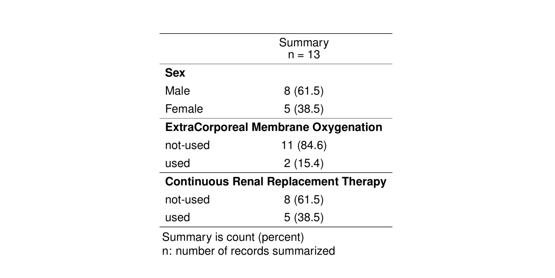
st_as_image(tab_cont)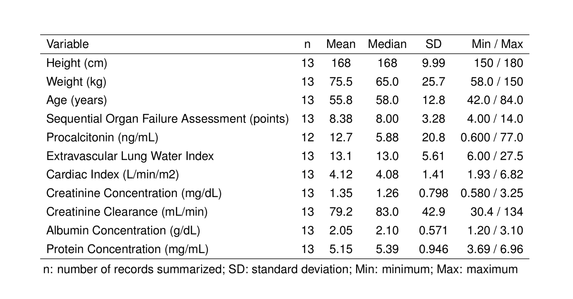
img_cat  <- image_read(here(table_dir, "Cat_table", "categorical_cov.png"))
img_cont <- image_read(here(table_dir, "Con_table", "continuous_cov.png"))
height <- min(image_info(img_cat)$height, image_info(img_cont)$height)
spacer <- image_blank(width = 100, height = height, color = "white")
img_combined <- image_append(c(img_cat, spacer, img_cont))

image_write(img_combined, here(table_dir, "combined_tables.png"))# namespace options
ys_namespace(spec)
specTex <- ys_namespace(spec, )
#filter your spec object
contCovDF <- ys_select(spec, c("BW", "AGE", "SOFA", "PCT", "ELWI", "CI", "CRE", "ALB", "PROTEIN"))
contCovNames <- names(contCovDF)
#axes labels
contCovarListTex <- axis_col_labs(specTex,
contCovNames,
title_case = TRUE,
short = 10)
dat <- xdata %>%
yspec_add_factors(spec,)
covar <- dat %>%
distinct(ID, .keep_all = TRUE)
ContVCont <- covar %>%
pairs_plot(y = contCovarListTex, diag = c("barDiag"),lower_fun = GGally::wrap("points")) +
theme(
axis.text = element_text(size = 6),
strip.text.x = element_text(size = 6),
strip.text.y = element_text(size = 4.5),
axis.title = element_text(size = 6)) +
rot_x(50)
ContVCont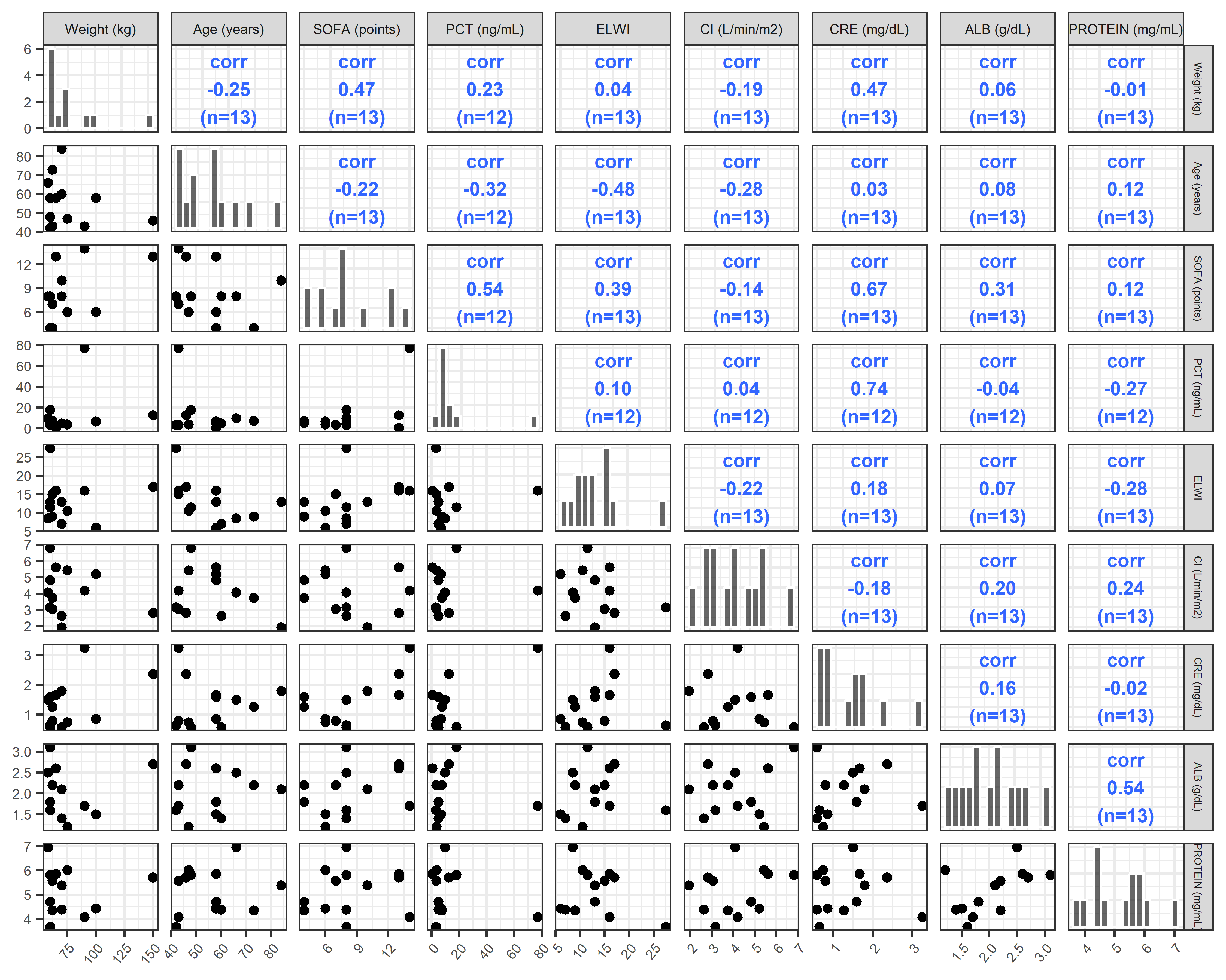
ggplot2::ggsave(ContVCont, filename = here::here("deliv/figures/EDA", "ContVCont.png"), width = 9, height = 7)ecmo_contCat_Total <- covar %>%
wrap_cont_cat(x = "ECMO_f//ExtraCorporeal Membrane Oxygenation",
y = contCovarListTex,
use_labels = TRUE)
ecmo_contCat_Total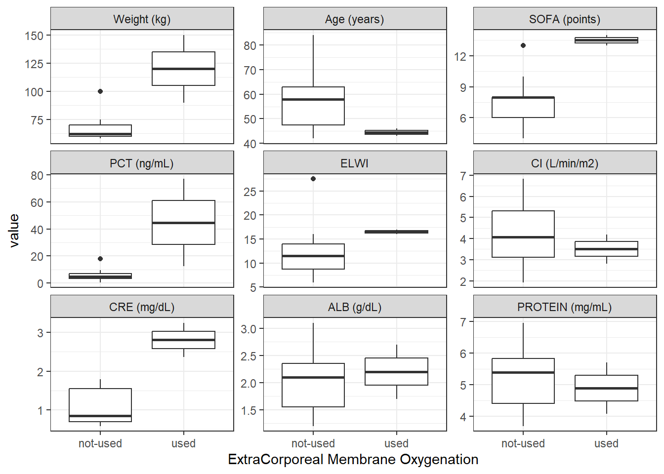
crrt_contCat_Total <- covar %>%
  wrap_cont_cat(x = "CRRT_f//Continuous Renal Replacement Therapy",
                y = contCovarListTex,
                use_labels = TRUE)


crrt_contCat_Total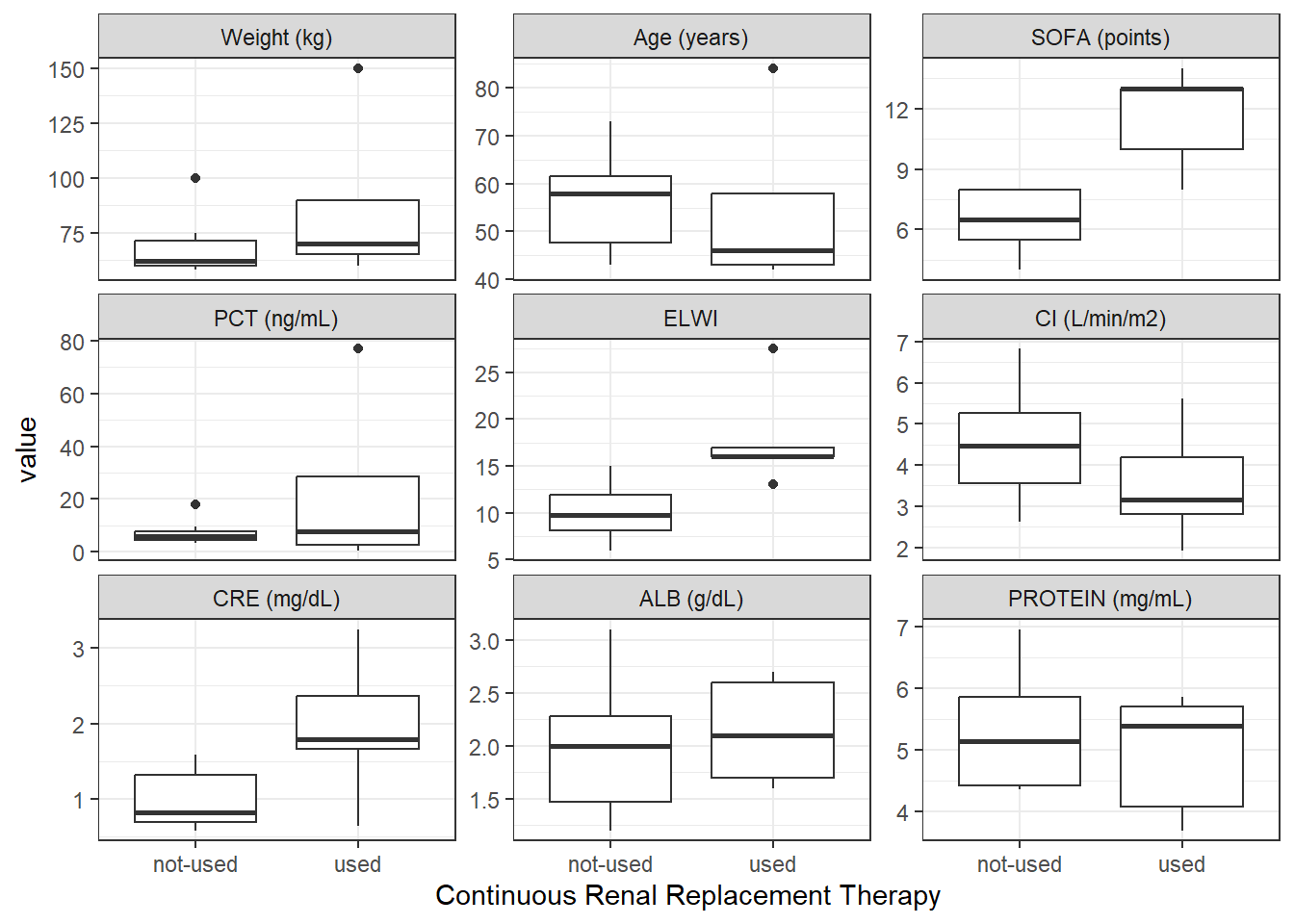
gender_contCat_Total <- covar %>%
  wrap_cont_cat(x = "SEX_f//Sex",
                y = contCovarListTex,
                use_labels = TRUE)

gender_contCat_Total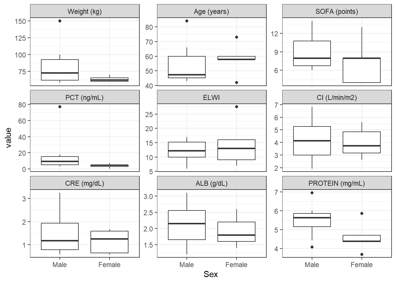
profiles <- map(unique(xdata$ID), function(u){
  temp <- xdata %>%
    filter(ID == u)

  ggplot(data = temp %>%
           filter(!is.na(DV) & EVID == 0), aes(TIME, as.numeric(DV), color = as_factor(CMT))) +
    geom_point(shape = 1) +
    geom_line(linewidth = 1) +
    geom_vline(data = temp %>%
                 filter(EVID == 1) %>%
                 mutate(t1 = TIME, t2 = TIME+II, t3 = TIME+II*2) %>%
                 pivot_longer(col=t1:t3, values_to = "bbb") %>%
                 filter(!c(ADDL==0 & name=="t2" | ADDL==0 & name=="3" | ADDL==1 & name=="t3")),
               aes(xintercept = bbb, col = "#fb9b06"),
               linetype = "dashed",
               alpha = 0.7) +
    scale_color_manual(values = c("bisque4", "deepskyblue4", "#fb9b06"),
                       labels = c("Ceftolozane", "Tazobactam", "Time of dose administration")) +
    scale_x_continuous(breaks = seq(0, 24, by = 4)) +
    labs(title = (paste0("Subject ", u, " PK Profile")),
         x = "Time after first dose (hours)",
         y = "Concentration (ug/mL)")
})

profiles
[[1]]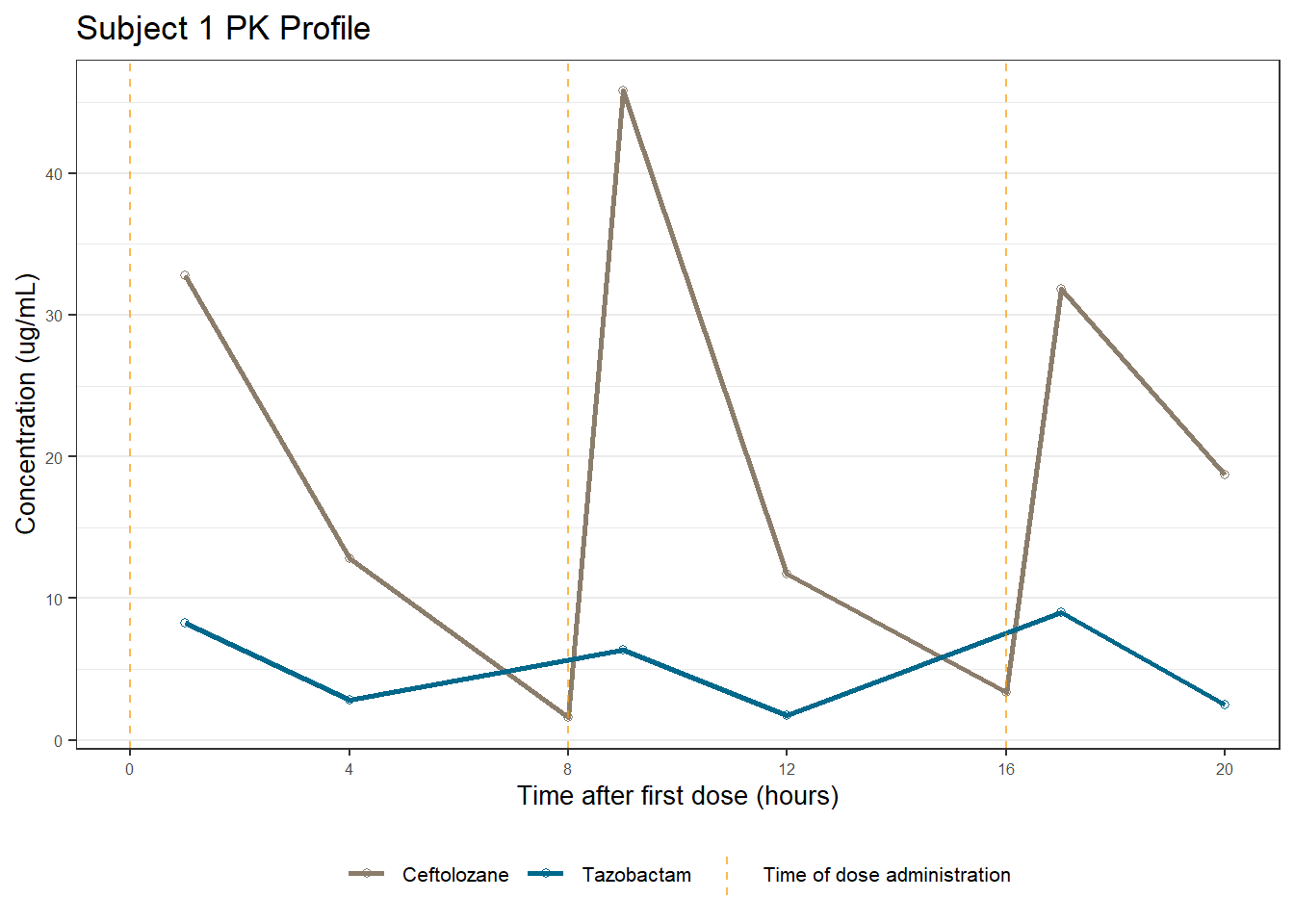
[[2]]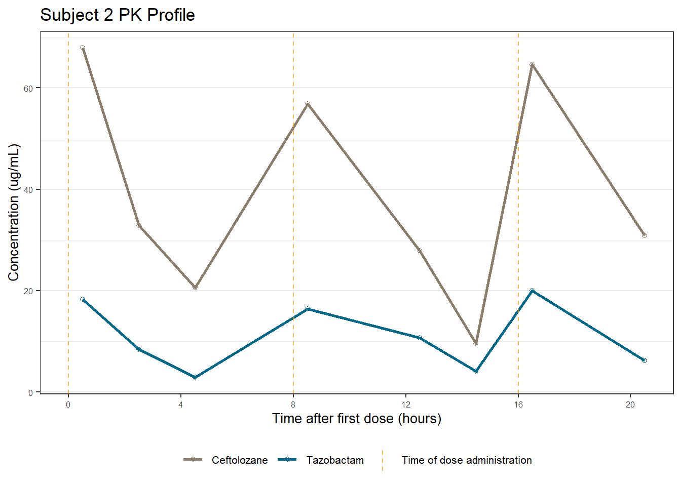
[[3]]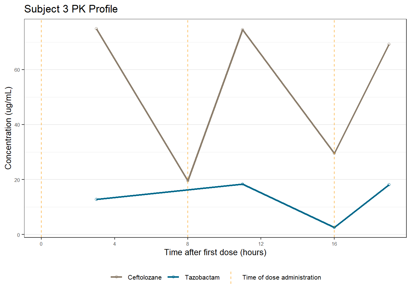
[[4]]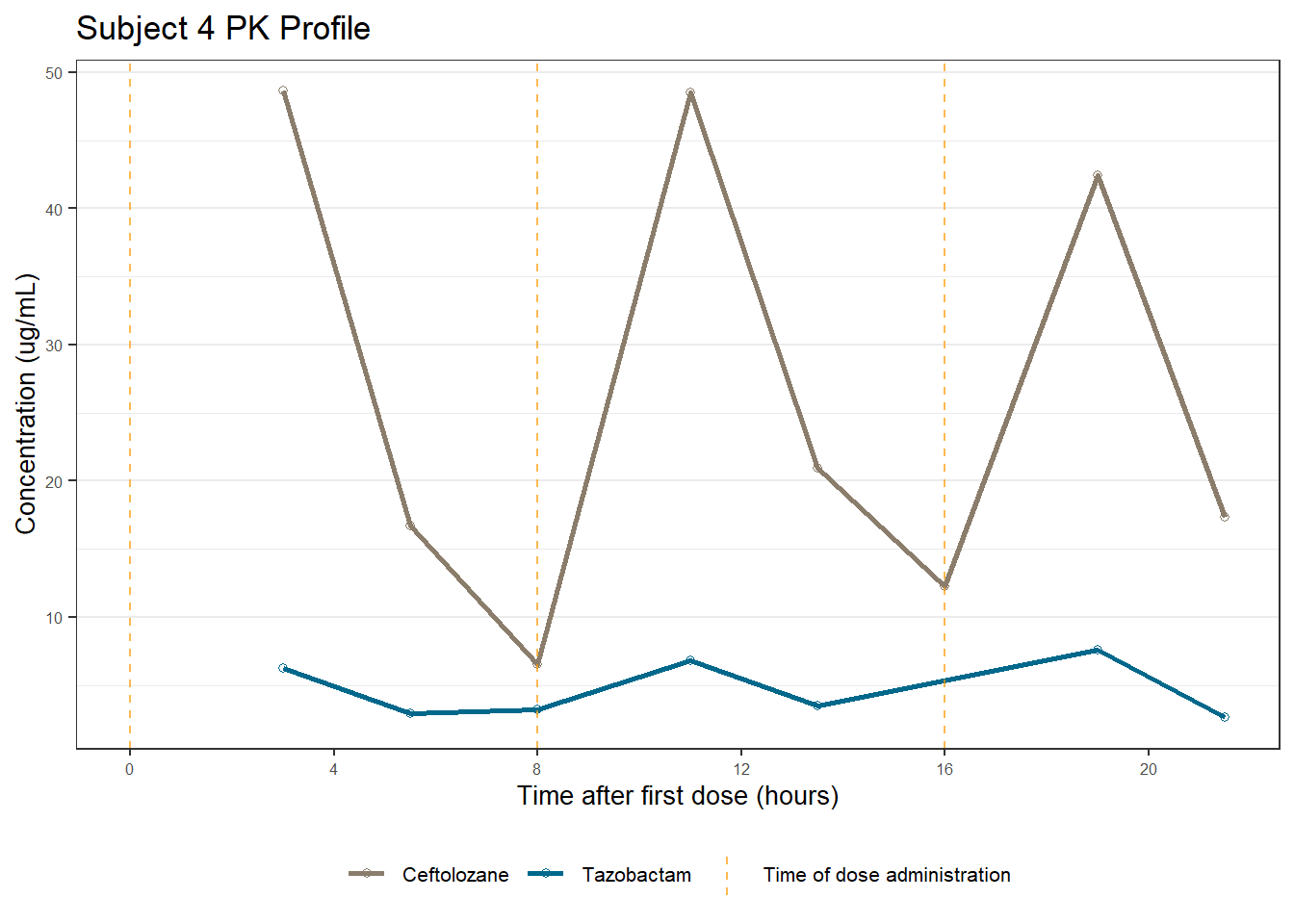
[[5]]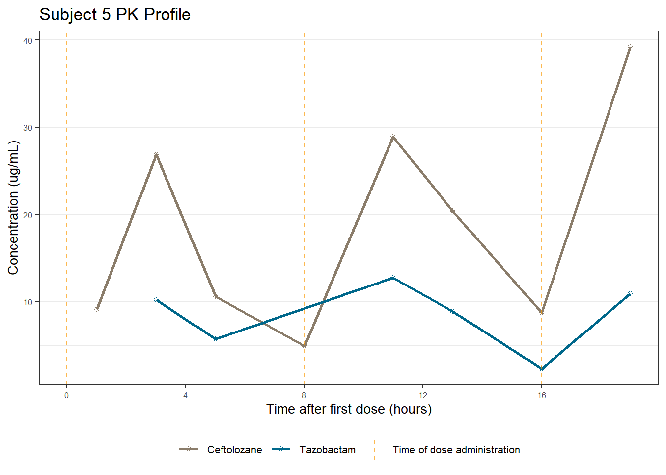
[[6]]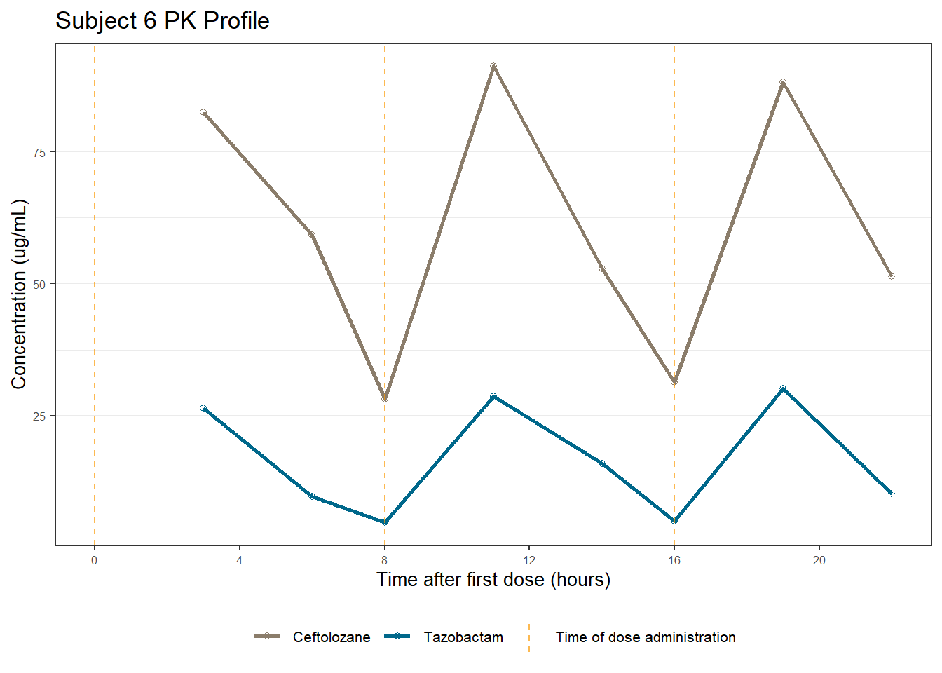
[[7]]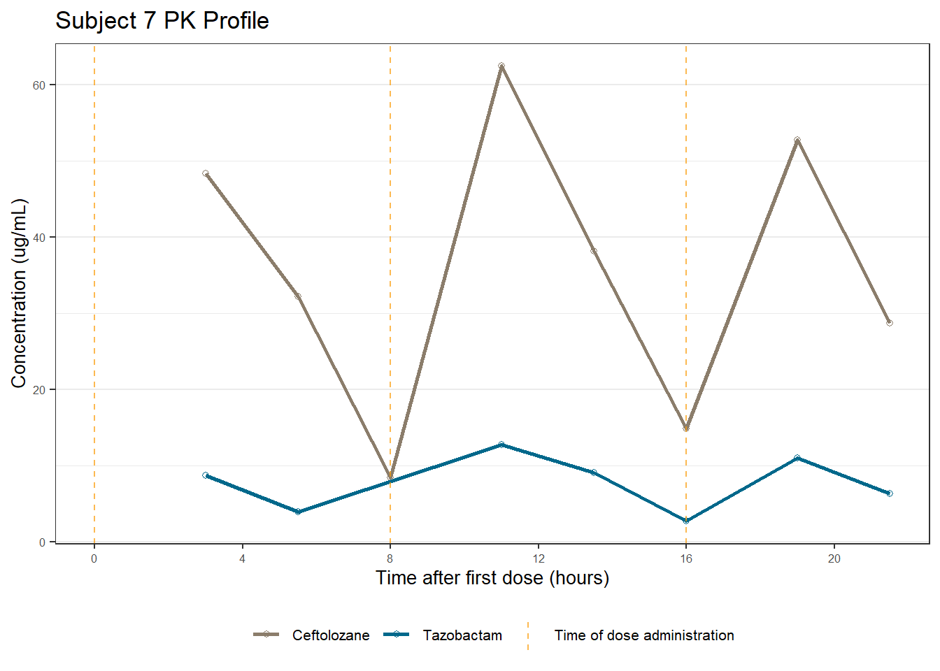
[[8]]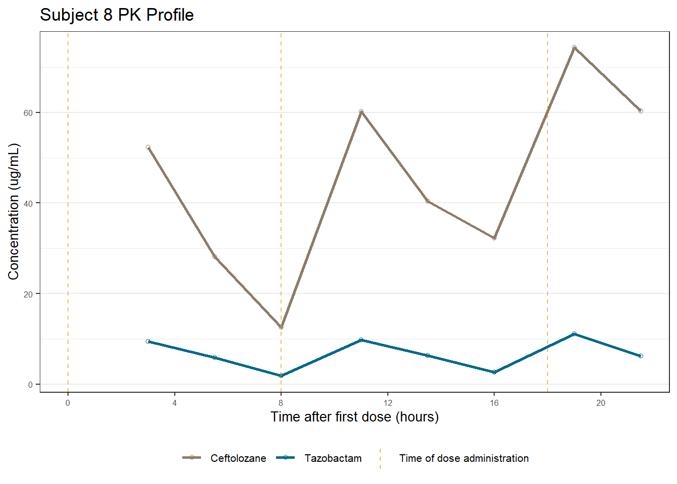
[[9]]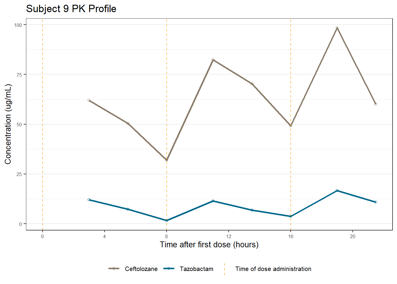
[[10]]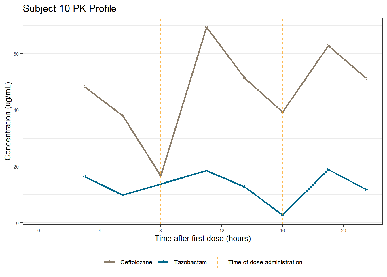
[[11]]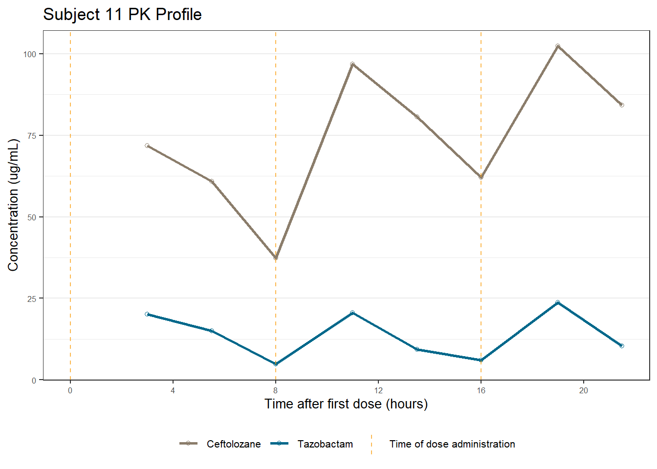
[[12]]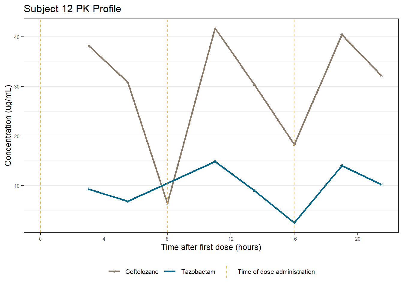
[[13]]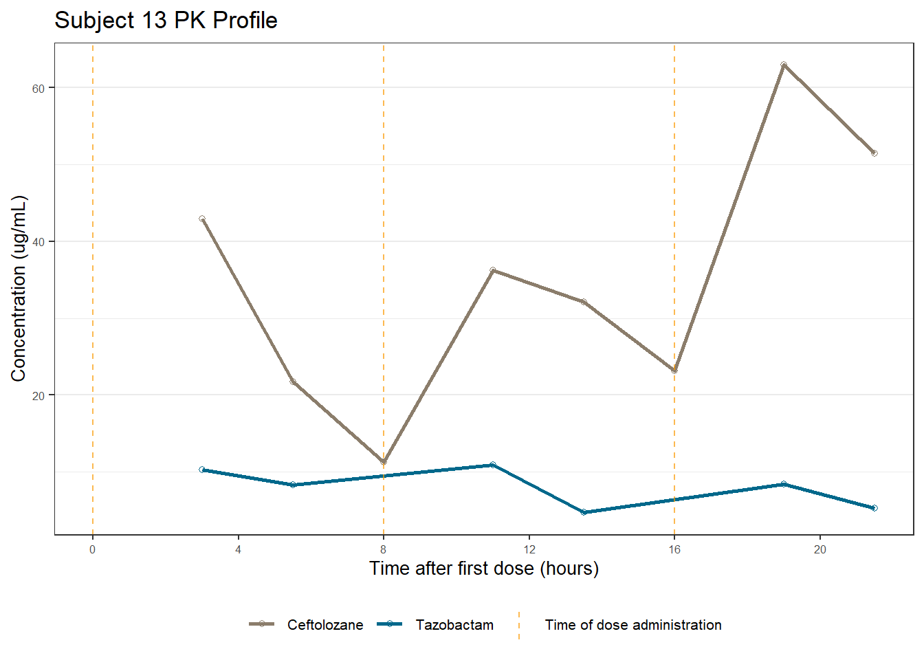
add_mg <- function(DOSEN) {
  paste(DOSEN, " mg")
}

ceftazlabel <- as_labeller(c("1" = "CEFTOLOZANE", "3" = "TAZOBACTAM"))plot1 <- ggplot(data = subset(xdata, EVID == 0), aes(x = TIME, y = DV, group = ID, color = as.factor(CMT))) +
geom_point() +
geom_point(colour = "grey33", alpha = 0.7) +
geom_line(data = subset(xdata, EVID == 0 & CMT == 1), aes(x = TIME, y = DV, group = ID), linewidth = 0.4) +
geom_line(data = subset(xdata, EVID == 0 & CMT == 3), aes(x = TIME, y = DV, group = ID), linewidth = 0.4) +
scale_y_log10()+
ylab("Concentrations, ug/ml") +
xlab("Time, h") +
theme(legend.position = "right") +
scale_x_continuous(breaks = seq(0, 24, by = 4)) +
scale_color_manual(labels = c("CEF", "TAZ"), values = c("bisque4", "deepskyblue4"))
print(plot1)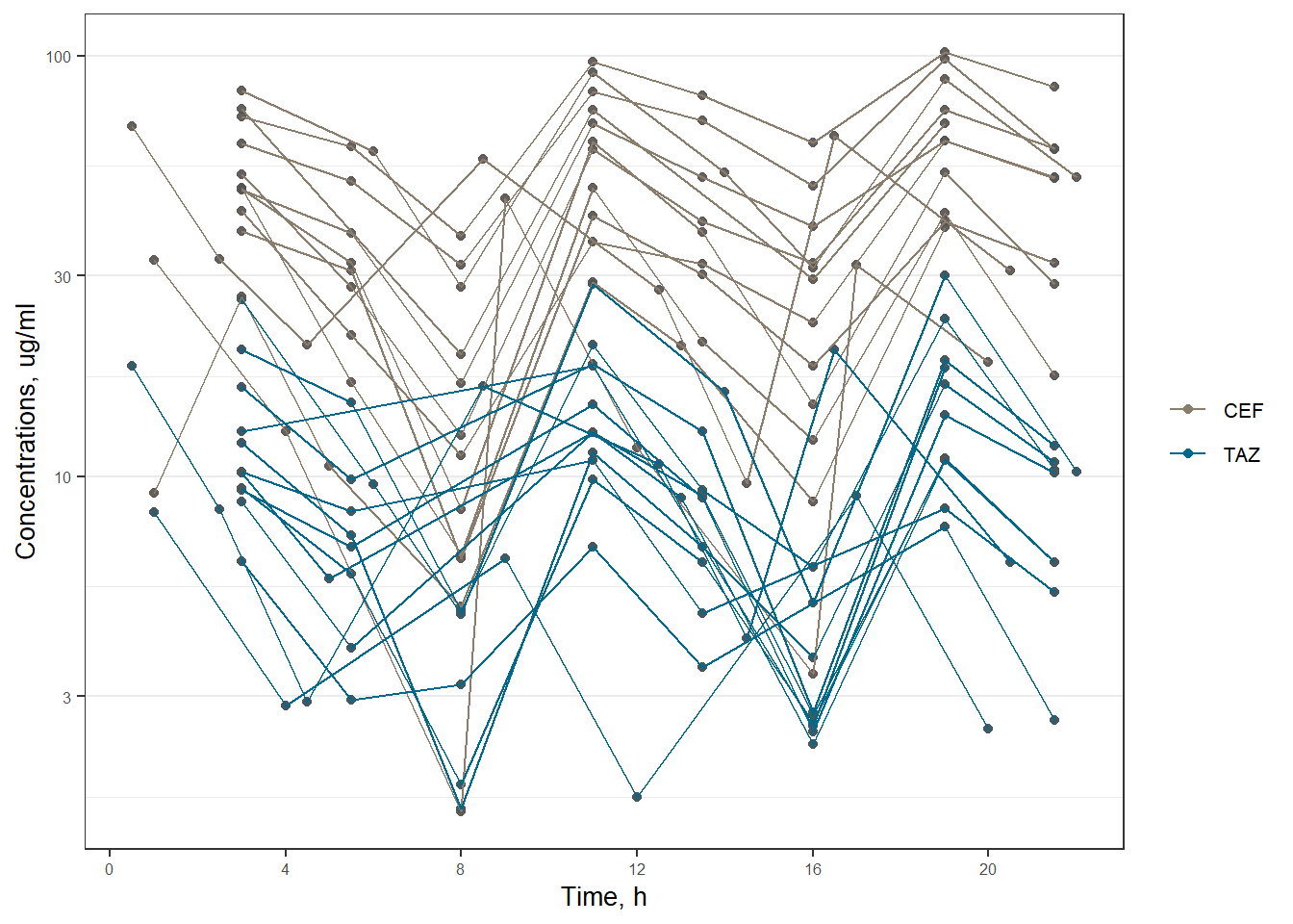
ggplot2::ggsave(plot1, filename = here::here(figure_dir, "rawdata1.png"), width = 12, height = 10, dpi = 600, units = "cm")plot2 <- ggplot(data = subset(xdata, EVID==0), aes(x = TIME, y = DV, color = factor(CMT)), shape = 21) +
geom_point(size = 0.6) +
geom_line(linewidth = 0.4) +
scale_y_log10()+
ylab("Concentrations, ug/ml") +
xlab("Time, h") +
labs(color = "ID")+
facet_wrap(.~factor(ID),nrow = 4) +
scale_x_continuous(breaks = seq(0, 24, by = 4)) +
scale_color_manual(labels = c("CEF", "TAZ"), values = c("bisque4", "deepskyblue4")) +
theme(legend.position = "right",strip.background = element_rect(fill = "grey95", color = NA),
strip.text = element_text(face = "plain") )
print(plot2)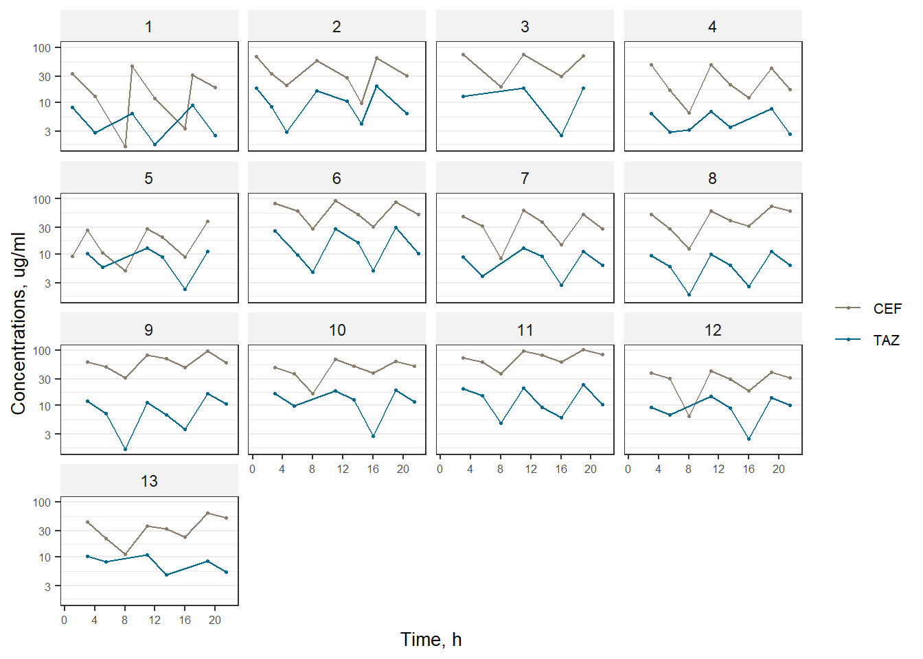
ggplot2::ggsave(plot2, filename = here::here(figure_dir, "rawdata2.png"), width = 12, height = 10, dpi = 600, units = "cm")cef_obs <- xdata %>%
filter(EVID == 0, CMT == 1) %>%
mutate(TIME_8H = TIME %% 8) %>%
group_by(TIME_8H) %>%
count()
taz_obs <- xdata %>%
filter(EVID == 0, CMT == 3) %>%
mutate(TIME_8H = TIME %% 8) %>%
group_by(TIME_8H) %>%
count()
left_join(cef_obs, taz_obs, by = "TIME_8H", suffix = c("_cef", "taz"))# A tibble: 11 × 3
# Groups: TIME_8H [11]
TIME_8H n_cef ntaz
<dbl> <int> <int>
1 0 24 14
2 0.5 3 3
3 1 4 3
4 2.5 1 1
5 3 33 33
6 4 3 3
7 4.5 3 3
8 5 2 2
9 5.5 24 24
10 6 3 3
11 6.5 1 1sessionInfo()R version 4.3.2 (2023-10-31 ucrt)
Platform: x86_64-w64-mingw32/x64 (64-bit)
Running under: Windows 11 x64 (build 26200)
Matrix products: default
locale:
[1] LC_COLLATE=Polish_Poland.utf8 LC_CTYPE=Polish_Poland.utf8
[3] LC_MONETARY=Polish_Poland.utf8 LC_NUMERIC=C
[5] LC_TIME=Polish_Poland.utf8
time zone: Europe/Warsaw
tzcode source: internal
attached base packages:
[1] stats graphics grDevices utils datasets methods base
other attached packages:
[1] webshot2_0.1.2 viridisLite_0.4.2 PKNCA_0.11.0
[4] Hmisc_5.2-1 pdftools_3.4.1 ggpubr_0.6.0
[7] GGally_2.2.1 mrggsave_0.4.5.9000 skimr_2.1.5
[10] kableExtra_1.4.0 conflicted_1.2.0 haven_2.5.4
[13] yspec_0.6.1.9000 arrow_18.1.0 magick_2.8.5
[16] yaml_2.3.8 magrittr_2.0.3 gridExtra_2.3
[19] cmdstanr_0.8.1.9000 nmrec_0.4.0 pmtables_0.6.0.9000
[22] pmplots_0.4.0.9001 scales_1.3.0 here_1.0.1
[25] whisker_0.4.1 glue_1.7.0 lubridate_1.9.3
[28] forcats_1.0.0 stringr_1.5.1 purrr_1.0.2
[31] readr_2.1.5 tidyr_1.3.1 tibble_3.2.1
[34] tidyverse_2.0.0 data.table_1.16.2 knitr_1.49
[37] naniar_1.1.0 mrgsolve_1.5.2.9000 patchwork_1.3.0
[40] ggplot2_3.5.1 dplyr_1.1.4 pracma_2.4.4
loaded via a namespace (and not attached):
[1] rlang_1.1.4 compiler_4.3.2 systemfonts_1.1.0
[4] vctrs_0.6.5 pkgconfig_2.0.3 crayon_1.5.3
[7] fastmap_1.2.0 backports_1.4.1 labeling_0.4.3
[10] promises_1.3.2 rmarkdown_2.29 tzdb_0.4.0
[13] ps_1.7.6 ragg_1.3.3 visdat_0.6.0
[16] bit_4.5.0.1 xfun_0.49 cachem_1.1.0
[19] jsonlite_1.8.8 later_1.4.1 parallel_4.3.2
[22] broom_1.0.7 cluster_2.1.6 R6_2.6.1
[25] stringi_1.8.4 RColorBrewer_1.1-3 rpart_4.1.23
[28] car_3.1-3 Rcpp_1.0.12 assertthat_0.2.1
[31] base64enc_0.1-3 nnet_7.3-19 timechange_0.3.0
[34] tidyselect_1.2.1 rstudioapi_0.17.1 abind_1.4-8
[37] websocket_1.4.2 processx_3.8.4 qpdf_1.3.4
[40] lattice_0.22-6 plyr_1.8.9 withr_3.0.2
[43] askpass_1.2.1 posterior_1.6.1 evaluate_1.0.1
[46] foreign_0.8-86 gridGraphics_0.5-1 ggstats_0.7.0
[49] xml2_1.3.6 pillar_1.10.2 carData_3.0-5
[52] tensorA_0.36.2.1 checkmate_2.3.1 renv_1.0.7
[55] distributional_0.5.0 generics_0.1.3 vroom_1.6.5
[58] rprojroot_2.0.4 chromote_0.5.1 hms_1.1.3
[61] munsell_0.5.1 xtable_1.8-4 tools_4.3.2
[64] ggsignif_0.6.4 fs_1.6.4 grid_4.3.2
[67] colorspace_2.1-0 nlme_3.1-164 repr_1.1.7
[70] htmlTable_2.4.3 Formula_1.2-5 cli_3.6.3
[73] textshaping_0.4.0 svglite_2.1.3 gtable_0.3.6
[76] rstatix_0.7.2 digest_0.6.37 htmlwidgets_1.6.4
[79] farver_2.1.2 memoise_2.0.1 htmltools_0.5.8.1
[82] lifecycle_1.0.4 bit64_4.5.2